How much information can a triangle give you? Well, if it’s on a CFD (‘Cumulative Flow Diagram’), then it appears to be quite a lot.
After sitting in a presentation recently, someone came up to me to ask how changes in WIP, Cycle Time and Delivery Rate alter the shape of a CFD. Specifically, how the shape of the triangle connecting these factors changes.
The basics
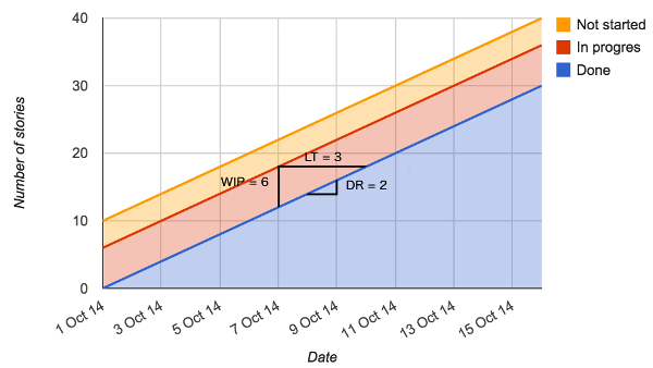
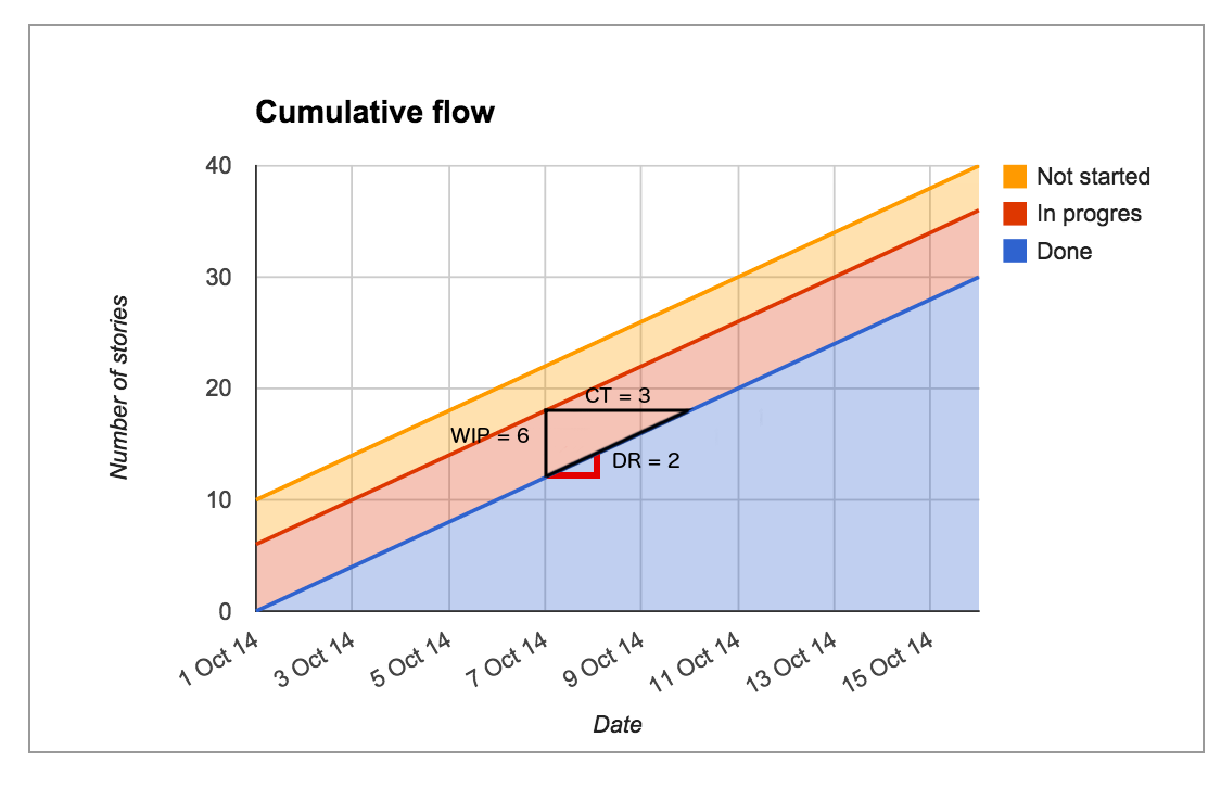
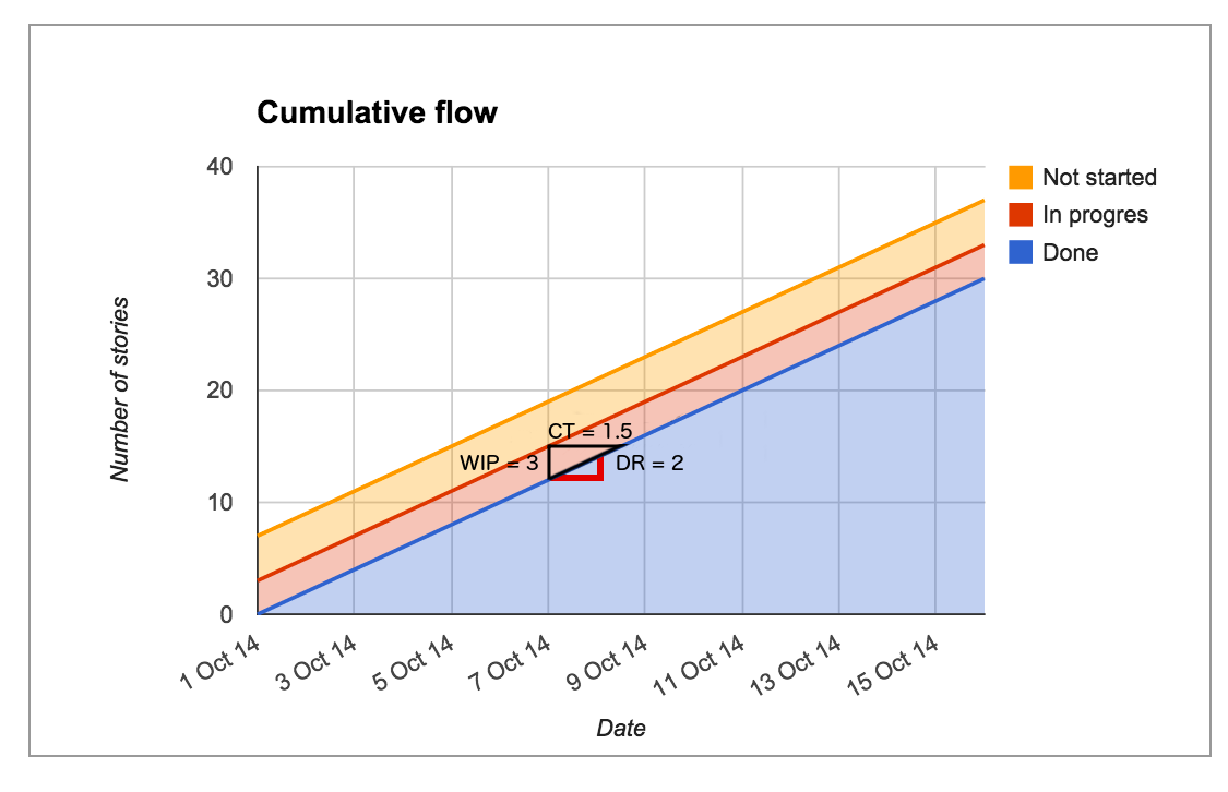
You can draw a triangle on your CFD to reveal how many work items you had in progress, your subsequent average cycle time*, and your delivery rate – for a snapshot in time.
For example, figure 1 shows that, on 7 October 2014, there were 6 items in progress, it took an average of 3 days for items to complete from that point, and 2 items were delivered in the subsequent 24 hours.
Not bad going for a couple of triangles.
A reminder of Little’s Law
As discussed in my previous post, Little’s Law tells us that if WIP, Cycle Time or Delivery Rate changes, at least one of the other elements will also be affected. Let me use our previous example to illustrate: if we reduce Cycle Time to 2 and keep WIP at 6, then Deliver Rate will change:
WIP / CT = DR
6 / 2 = 3
How does that change the CFD?
And this is where we come back to my conversation about the shape of the triangle. If we change Cycle Time and Delivery Rate as described above, then our CFD would look like this:
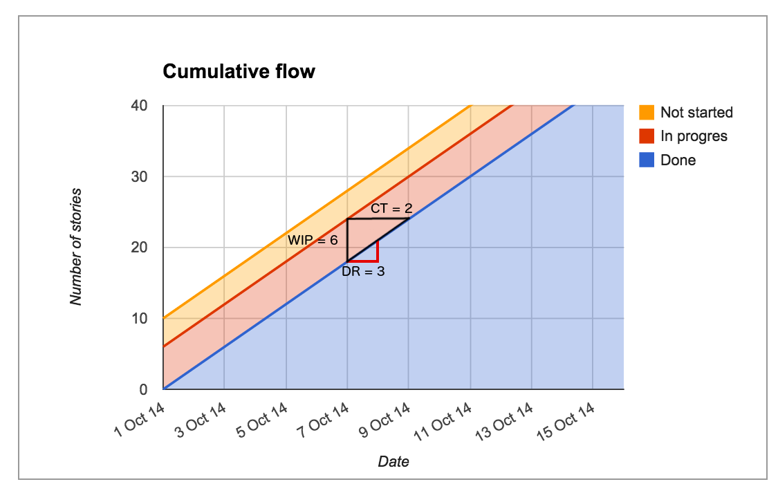
You will notice that the hypotenuse (the longest side of the triangle) in figure 2 is steeper than in figure 1. In essence, you can see how Delivery Rate has improved just by comparing the hypotenuse on a CFD:
Does reducing WIP always improve Delivery Rate?
Mathematically, no. Little’s Law says DR = WIP / CT. So, if you reduced WIP but keep Cycle Time constant, then Delivery Rate actually worsens. In the real world, if you work on fewer items (i.e. reduce WIP) then your Cycle Time will normally reduce.
However, if you change two values but keep their ratios the same, then the third value will remain unchanged. For example, if we take our first example and halve the WIP to 3 and halve the Cycle Time to 1.5 days, then we would still end up with a Delivery Rate of 2 items per day:
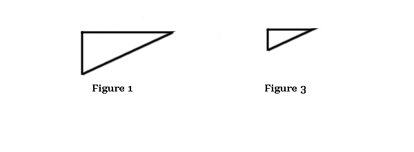
What you might notice in our last chart, is that its triangle, albeit bigger in area, is the same shape as figure 1. The same shape of the triangle means the delivery rate is the same.
Conclusion
Of course, what we are really talking about here is the angle in that bottom corner. But, you don’t need to dust of your trigonometry knowledge to see what is going on here; if the longest side of the triangle is getting steeper, then your Delivery Rate is improving.
This isn’t ground-breaking mathematics, but it’s another clue that CFDs hold about our flow. CFDs really are a marvellous tool.
* I use Cycle Time rather than Lead Time because I’m referring to only part of the process
Great post. Addresses some of my concerns that Little’s Law is sometimes used inappropriately. For example, according to the Law, if I want to dramatically increase my Delivery Rate, I could keep the same Cycle Time and just triple the Work In Progress…
But the important point, for me, is that assuming we’re not sure how changes might affect DR, reducing the WIP will *most likely* reduce the CT. And a reduced CT has, in and of itself, significant benefits: quicker to market; quicker feedback; fail faster etc.
PS nothing wrong with a bit of SOHCAHTOA now and then.
You and your SOHCAHTOA 🙂
Another way to look at this, is taking into account that in a queue that is used to process work (dependent events) there is one step that is taking longer than the others. A lot has been said about this in the Theory of Constraints knowledge regarding operations, and the explanation of Drum-Buffer-Rope method to address that step. When you take Little’s Law into account, and you say that only a limited amount of work can pass through the constrained step – the maximum potential throughput of the whole system as a whole can be determined. Once you have the maximum throughput, it makes no sense to compromise on less throughput but it also makes no sense to keep increasing the Work in Process which will just increase Lead Time while the maximum throughput has already been reached. I created a simulation in Google Sheets that shows this at http://dvps.me/toc-littles-law