Introduction
In 1908, a guy at Guinness found a way to measure which types of barley produced the best beer-brewing yields: he called it the “t-statistic”. However, because Guinness was paranoid about giving away trade secrets, he had to publish his ideas under the pseudonym “Student”. Although we now know his name was William Sealy Gosset, his idea is still known as Student’s t-statistic.
In short, Gosset believed that you could take a small amount of data and use it to forecast the future … if you take the appropriate level of error into account.
An example
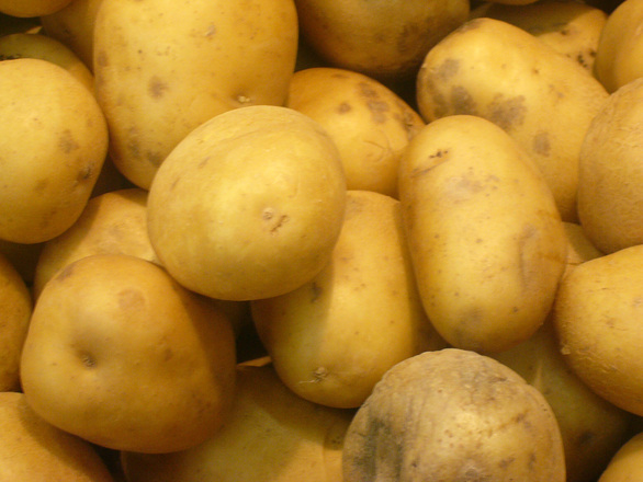
For example, if we take 2 potatoes, we can calculate the range that a third potato will fall between. We tried it at Agile on the Beach last week and this is what happened:
- The first potato weighed 159 grams
- The second potato weighed 170 grams
- That is an average weight of 164.5
- Subtract the average from each data sample, then square the result of each: (159-164.5)2 + (170-164.5)2
- Add all the squares together: 30.25 + 30.25 = 60.5
- Divide by 1 less than number of samples: 60.5 / 1 = 60.5
- Divide by number of samples: 60.5 / 2 = 30.25
- Square root: √ 30.25 = 5.5 [note 1]
- Multiply by relevant T-stat (for 2 samples, this is 6.31) to get the sample error: 5.5 x 6.31 = 34.7
- Subtract the sample error from the average to calculate the lower bound: 164.5 – 34.7 = 129.8
- Add the sample error to the average to calculate the upper bound: 164.5 + 34.7 = 199.2
- So, in our in-talk example resulted, did the third potato fall between 130 and 199? Yes: the third spud came in at 175 grams.
We could now repeat the equation with three data samples. This would now use the t-statistic of 2.92 as the margin of error decreases with more data samples (down to 1.645 for large samples).
Does it work?
The beauty of this is that our data sample is small, yet we are accounting for sample variation. The problem is, it assumes a normal distribution. So if your data has any other distribution (such as most software projects which have a weibull distribution), it has the potential for going pretty badly.
I ran over 10 tests for various topics (ranging from time it took to be served a coffee to track length of tunes on a Spotify playlist) and found that the results varied wildly depending on the type of data set. Overall the success rate was between 40% and 50%, but it worked better for some data types (e.g. track length of tunes and train journey times) than others (e.g. distance walked per day, shoe sizes of people in a crowd, duration of tennis matches at Wimbledon). Across the board, smaller data samples were more successful than larger data sets.
Gosset’s error margins decrease as you have more data points. This may sound familiar as it is the basis of the cone of uncertainty. Also, the flattening of the cone illustrates that taking more samples is less rewarding: you need to increase your samples by a large amount to increase the chances of more accurate data so, often, the cost of increasing your sample size has diminishing returns.
Conclusion
Student’s t-statistic works quite well for small data samples, but it does return a large range. It also doesn’t work very well for larger data samples.
However, if our aim is to “reduce uncertainty”, then this may be an effective, quick method. You’d need to see if it works for you.
NOTE 1: the calculation up to here is a bit silly when you have just 2 data samples, but I included the steps that you need to perform with 3+ data points.
Photo credit (homepage): Barbara Bar
